An Analysis of Median Finding Algorithms

In this assignment, we will be studying the problem of finding the median element of an array with n elements. To do so, we will inspect three different algorithms, and analyze their time complexities, characteristics, advantages and disadvantages.

Algorithm 1

In this algorithm, what we are trying to achieve is to move the biggest (n + 1)/ 2 elements of the array to the beginning of the array. In this case, the median of the element becomes the (n + 1)/2 th element in the array, which has index (n - 1) / 2.

To do so, in each iteration in the for loop, we search for the maximum element in the array. To obtain the biggest (n + 1) / 2 elements, in the worst case, we need to iterate through the outer loop (n + 1) / 2 times, and for the inner loop, we iterate (n - 1) times at first iteration of the while loop, (n - 2) times at second iteration of the while loop … and (n - (n + 1) / 2) times at (n + 1) / 2 th iteration of the while loop.

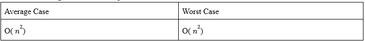
As we can see, for both the inner and outer loops, we have the time complexity in order of n. As we know that the total running time of a statement inside a group of nested loops is the running time of the statement multiplied by the product of the sizes of all the loops, we can say that the Big-Oh notation for the worst case of the function is: O( 𝑛^2 )

In the average case, we again need to iterate through the outer loop (n+1) / 2 times, and for the inner loop, we iterate the same amount. This is because the number of iterations of the loops are fixed for the value of n. As we know that the total running time of a statement inside a group of nested loops is the running time of the statement multiplied by the product of the sizes of all the loops, we can say that the Big-Oh notation for the average case of the function is: O( 𝑛^2 )

So, for the first algorithm, time complexities are:

The code for the first algorithm can be seen below:

int FIND_MEDIAN_1( int input[], const int n) {
    int maxIndex, maxValue;
    int count = 0;
    while(count < (n+1)/2) {
        maxIndex = count;
        maxValue = input[count];
        for( int j = count+1; j < n; j++ ) {
        if( input[j] >= maxValue ) {
            maxIndex = j;
            maxValue = input[j];
        }
    }
    swap( input[count], input[maxIndex] );
    count++;
    } 
    return input[count-1];
}

void swap( int &n1, int &n2 ) {
    int temp = n1;
    n1 = n2;
    n2 = temp;
} 

-

Algorithm 2

In the second algorithm, the implementation is similar, but we sort the whole array this time.

In this algorithm, we first have to sort the whole array in a descending order with the randomized quick-sort algorithm. We call this quick-sort algorithm randomized because we choose the pivot index randomly.

Now, let’s inspect this randomized quick-sort algorithm. We should start by noticing that this algorithm works recursively, that is, it calls itself again and again until the array is fully sorted. After fully sorting the array, we will see that the median of the array is the middle element of the array, which is the (n + 1)/2 th element of the array at the (n - 1)/2 th index.

In this algorithm, the worst case occurs when the pivot is the minimum or the maximum of the array. In this case, an array of n elements will be parted into n - 1 element and 1 element parts. Then, the n - 1 element array will be parted into n - 2 element and 1 element parts and so on. In each recursive call, the array which the function was called on will go through the for loop, and this for loop will iterate for n’ times, where n’ is the size of the array. In the for loop, there will be a constant number of operations, say C.

T( n ) = T ( n - 1 ) + ( C * n )

T( n ) = T ( n - 2 ) + ( C * n ) + ( C * (n - 1) )

T( n ) = T ( n - 3 ) + ( C * n ) + ( C * (n - 1) ) + ( C * (n - 2) ) … T( n ) = T( 1 ) + ( C * n ) + ( C * (n - 1) ) + … + ( C * 2 )

T( n ) = T( 0 ) + ( C * n ) + ( C * (n - 1) ) + … + ( C * 2 ) + ( C * 1 )

Then, T( n ) = C [ ( n ) + ( n - 1 ) + … + 1 ] = C * [ (( n ) * ( n + 1)) / 2 ] = C/2 * [ 𝑛^2 + n]

As we can see here, the time complexity is in the order of 𝑛 . So, the Big-Oh notation for the worst case of the 2 function is: O( n^2 )

In the average case, an array of n elements will not be parted into n - 1 element and 1 element parts, but rather two n /2 element parts, and in each recursive call, the array which the function was called on will go through the for loop, and this for loop will iterate for n’ times, where n’ is the size of the array. In the for loop there will be a constant number of operations, say C.

T( n ) = T( n / 2 ) + ( C * n )

T( n ) = T( n / 4 ) + ( C * n ) + ( C * (n / 2) )

T( n ) = T( n / 8 ) + ( C * n ) + ( C * (n / 2) ) + ( C * (n / 4) ) … T( n ) = T( 0 ) + ( C * n ) + ( C * (n / 2) ) + ( C * (n / 4) ) + … + ( C * 1 )

Then, T( n ) = ( C * n ) + ( C * (n / 2) ) + ( C * (n / 4) ) + … + ( C * 1 )

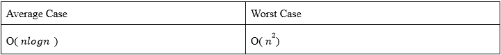
As we can see here, we will call the function 𝑙𝑜𝑔 𝑛 times, and at each call, the for loop will iterate in the order of 𝑛 times. So, the Big-Oh notation for the average case of the function is: O( 𝑛𝑙𝑜𝑔𝑛 )

So, for the second algorithm, time complexities are:

The code for the second algorithm can be seen below:

int FIND_MEDIAN_2(int input[], const int n) {
    randomizedQuickSort(input, 0, n - 1 );
    return input[(n-1)/2];
}

void randomizedQuickSort(int input[], int p, int r) {
    int q;
    if( p < r ) {
        q = randomizedPartition( input, p, r );
        randomizedQuickSort( input, p, q - 1 );
        randomizedQuickSort( input, q + 1, r );
    }
}

void swap( int &n1, int &n2 ) {
    int temp = n1;
    n1 = n2;
    n2 = temp;
}

int randomizedPartition( int input[], int p, int r ) {
    int index = rand() % (r-p+1) + p;
    swap(input[index], input[r]);
    int x = input[r];
    int i = p - 1;
    for( int j = p; j < r; j++ ) {
    if( input[ j ] >= x ) {
        i = i + 1;
        swap( input[i], input[j]);
        }
    }
    swap(input[i+1], input[r]);
    return i + 1;
}

-

Algorithm 3

In the third algorithm, the pivot will not be chosen randomly, but in a more complicated manner, by calling itself recursively in a random sample of the input.

The problem with the randomized quick-sort algorithm was that we could pick really bad pivot points. We want to pick a pivot that is reasonably close to the median really quickly. The way to do this is instead of trying to find the median of the whole set, finding the median of subsets and then finding the median of these medians. This way, we can reach our goal of finding the median of the whole array just by looking at the median of the medians.

To apply this algorithm, we should partition the array in groups of 5, so we will have n / 5 such partitions in total. Now, for each partition, we can find the median of that partition in 6 steps, so we go through 6n / 5 such steps to find all of the partitions’ medians.

Now, to find the median of these medians, we write a recurrence relation. If T( n ) is the time required to run the algorithm on n elements, then we have n / 5 medians, and the time required is T ( n / 5 ). Let M be the median of medians in this algorithm. Now that we have found the median value M, among the n / 5 elements, we have n / 10 larger elements than M, and n / 10 smaller elements than M. And as each one of these elements is greater or less than at least two elements on this list, the true median is greater than and less than at least 3n / 10 element in the list. By the symmetry, there are at least 3n / 10 values greater than M, and at least 3n / 10 values less than M. So, the final recursive call is on a list of at most 7n / 10 elements and takes time at most T ( 7n / 10 ).

We can show these recursive calls as: T(n) = T(n / 5) + T(7n / 10) + dn, and we want to show that T(n) is in linear time; we can do this by induction:

Induction Hypothesis: Assume that T(n) ≤ k * n, for some constant k.

Base Case: T(1) = c ≤ k . 1 therefore k ≥ c

Inductive Case: We can write T(n) as ( n / 5 ) * k + ( 7n / 10 ) * k + d * n; and we have T(n) = 9kn / 10 + dn ≤ kn for some number k ≥ 10d, and thus we showed that T(n) is indeed in linear time.

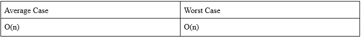
So, the Big-Oh notation for the worst case of the function is: O(n)

So, for the third algorithm, time complexity is:

The code for the third algorithm can be seen below:

int FIND_MEDIAN_3( int input[], const int n) {
    return select(input, n, (n+1)/2, 0, n - 1, 0 );
}

int select( int input[], int n, int k, int start, int end, int flag ) {
    if( n <= 5 ) {
        quickSort( input, start, end );
        return input[ start + k - 1 ];
    } 
    int i = start, numGroups = (int) ceil( ( double ) n / 5 ), numElements, j = 0;

    int *medians = new int[numGroups];

    while( i <= end ) {
        numElements = findMin( 5, end - i + 1 );
        medians[( i - start ) / 5] = select( input, numElements, (int) ceil( ( double ) numElements / 2 ), i, i + numElements - 1, 1 );
        i = i + 5;
    } 
    int M = select( medians, numGroups, ( int) ceil( ( double ) numGroups / 2 ), 0, numGroups - 1, 1 );
    delete[] medians;
    if( flag == 1 )
        return M;

    int q = partition( input, M, start, end );
    int m = q - start + 1;

    if( k == m )
        return M;
    else if( k < m )
        return select( input, m - 1, k, start, q - 1, 0 );
    else
        return select( input, end - q, k - m, q + 1, end, 0 );
}

Tables

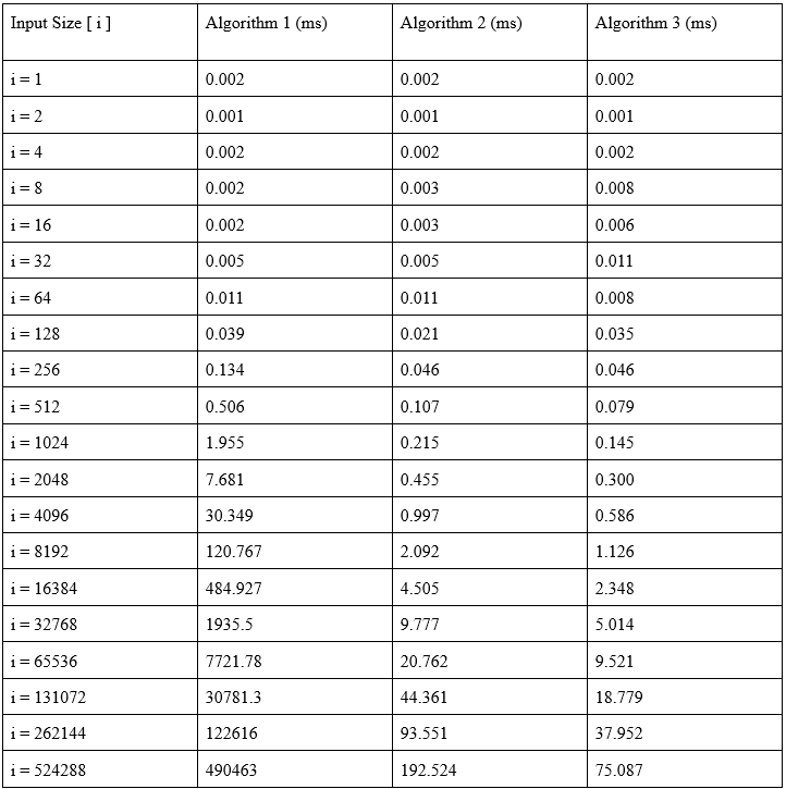
Below are the execution times of different algorithms for 20 different input sizes.

Plots

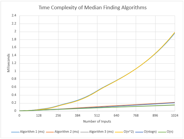
Discussion

In the benchmark we have created, we can see that the expected growth rates and the obtained results are very similar. The first algorithm runs on O( 𝑛^2 ) at average case and the worst case, whereas the second 2 algorithm runs on O( 𝑛𝑙𝑜𝑔𝑛 ) at average case and O( 𝑛^2 ) at worst case, and the third algoritm runs on O( n ) in the worst case. Looking at these time complexities, it is expected that the fastest algorithm is the third algorithm, and the slowest algorithm is the first algorithm. In the result we have obtained, we can see this more clearly. For all input sizes, execution time of algorithm one was bigger than execution time of algorithm two, and the execution time of algorithm two was bigger than algorithm three. We should also inspect the increase in the execution times related to input sizes. For the first algorithm, we can see that every time input size doubles, the execution time almost always goes up to four times its previous value because the worst and average cases are both in the order of 𝑛^2 . For the second algorithm, the average case is in the order of nlogn and as the logarithms grow slowly, we should expect a nearly-linear increase in the execution times, that is, when the input size doubles the execution time should double. However, as the worst case is in the order of 𝑛^2 , the increase in the execution times may not be linear in some boundary cases, but still we have a nearly linear graph as such cases occur rarely. For the third algorithm, as the worst and average time complexity is in the order of n, we expect that every time input size doubles, the execution time will double, which is what we see when we inspect the data and the graph we have obtained. We have previously said that the second and third algorithms are faster than the first algorithm. When we look at the results we have obtained and the plotted graphs, we can see the major difference between the execution times. These data we have obtained alone is sufficient to demonstrate that the choice of algorithms and efficiency are really important when working with large input sizes. While we could still deal with larger input sizes with the second and third algorithms, the first algorithm would be much slower and basically useless in such situations. So, whenever possible, it is best to search for the best algorithm for our purposes and use it instead of using the same algorithms over and over again. Lastly, in our observations, we see that algorithms acted differently for different input sizes, and it is even possible that for larger input sizes the algorithm can find the median faster. This may be caused by the arrangement of the array elements, that is, some arrangements can favor one kind of algorithm, and cause the worst-case in the other algorithms. It can also be that the momentary RAM usage of the development environment can change, thus the execution times are affected. In either case, we can test these algorithms more fairly by doing these observations over and over again to avoid sampling bias and get the most accurate results. The computer specifications hold a great importance, however in this case the CPU and the RAM usage were limited by the IDE, so we would get similar results with a slightly weaker computer.